This might come as a surprise, but I believe that data and analytics tools don’t have to live exclusively with data analysts. Everyone, from directors and managers to households, can use commands in Excel or Google Sheets to perform everyday tasks. All it takes is the knowledge and skillset to know what to input and how to sort the data so you can quickly find the answers you need.

I know how powerful this can be for non-data analysts because I’ve worked with people in many different roles outside the data team. Each time we come up with a new command, I see their eyes opening up and I can feel their sigh of relief in that they no longer have to spend hours searching for insights. The easy-to-setup commands can do that tedious work for them.
To help you feel that same sense of clarity and relief from the data you have at your disposal, here are four commands I’ve used to help navigate the business world for non-data analysts.
#1: XLOOKUP
There are countless examples when you might want to look up another record on another cell in a spreadsheet. For example, there may be an instance where you need to see inventory for one of your SKUs from a specific supplier. Or, you might want to look at the performance of a specific sales channel. In those instances, using XLOOKUP is your new go-to command.
In the past, many people used VLOOKUP to find certain data points, such as addresses or names. However, there were certain limitations with that code. XLOOKUP is the new and improved command you’ll want to use as you navigate your columns and rows of data.
To perform this command, choose the cell where you want the new data to appear and type “=XLOOKUP(lookup, lookup_array, return_array, not_found, match_mode, search_mode)”
- lookup refers to what you’re searching for
- lookup array or return array refers to the area where you want to search
- The remaining commands in italics are what you can tell Excel or Google Sheets to post if a match is not found or there’s a match.
Here’s an example of how a private tutor can use XLOOKUP to determine how many hours he/she worked for a specific date.
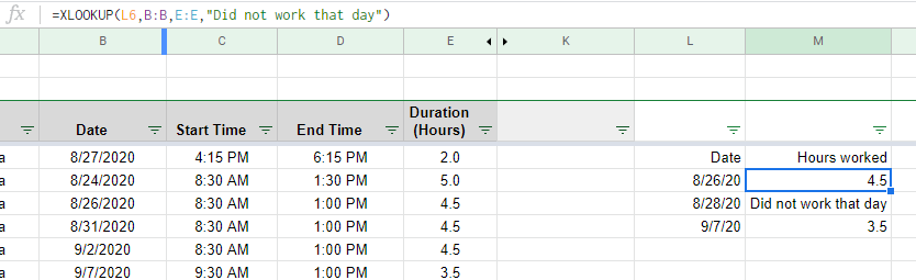
In this example, you can see that lookup was Cell L6, lookup_array was Column B (Date), and return_array was Column E (Duration(Hours)). The not_found was “Did not work that day,” so I asked the formula to return “Did not work that day” if a match is not found.
Application: I like this approach because XLOOKUP can look horizontally and vertically, which means you have a lot of flexibility in using this command. The use cases are plentiful from finding addresses for specific people or hours worked on specific days.
#2: Filtering
The above command allows you to pull up a specific result. However, there are times when you may want to have multiple records returned. That’s where using the filter command comes into play.
A filter command allows you to take a range from one column and filter out the information within that column. To do this, you would use this command: “=FILTER(array, include, [if_empty]).”
In our restaurant example, a filter would be useful when tracking how long employees take breaks.
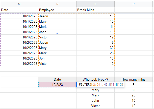
In the example, the array, or the dataset we want to filter for, was N2:O11, and the condition, or the number of minutes we wanted to look for, was M2:M11=N15. In this example, Mary and Mark take more time on their break than the rest of the employees.
Application: Using a filtered image, you can identify key information about a specific area of your business. For example, as a restaurant owner, you can monitor which employees take longer breaks and which might not take enough breaks throughout their shifts.
#3: Two-Way Lookup
Two-way lookup is similar to the XLOOKUP command mentioned above in that it looks up data. However, the two-way lookup command lets you analyze further, comparing two separate rows and columns to find the data you’re looking for.
To use this command, select a section in your spreadsheet where you can have three cells.
- The first cell would include your first lookup criteria (vertically).
- The second cell would include your second lookup criteria (horizontally).
- The third cell would be a combination of both XLOOKUP and FILTER functions.
Using a restaurant example, let’s consider an instance when a restaurant owner would want to determine the number of hours an employee worked on a specific day. To do that, he’d use a two-way lookup function. In the first cell, he’d select the employee’s name. In the second cell, he’d select the date. Here’s what it looks like in action:
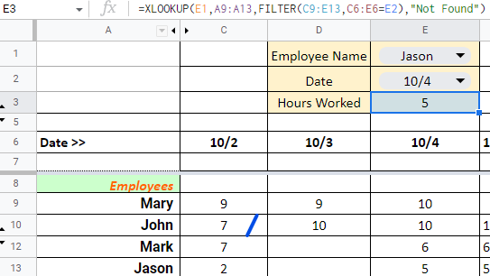
In the third cell, we get the result that shows that Jason (our first search criterion) worked on October 4 (our second search criterion) for 5 hours (the result we were looking to get from this command).
In the above example, within the XLOOKUP function, you can see that lookup was Cell E1, lookup_array was A9:A13 (Employee’s Name), and return_array was a FILTER function where the range was C9:E13 (make sure the row range matches the XLOOKUP lookup_array), and the condition was C6:E6=E2 (to find the matching date).
Application: By using the two-way lookup, managers and directors can make it faster and easier to find specific data in a hurry rather than always sifting, scrolling, or using the CTRL+F function to find one data criterion.
#4: Stacking Columns
There are times when you receive a file that has been formatted with data across multiple columns. When it comes time to use the commands above, or when you want to consolidate a variety of data points into one column, you’ll want to use the stacking column functionality.
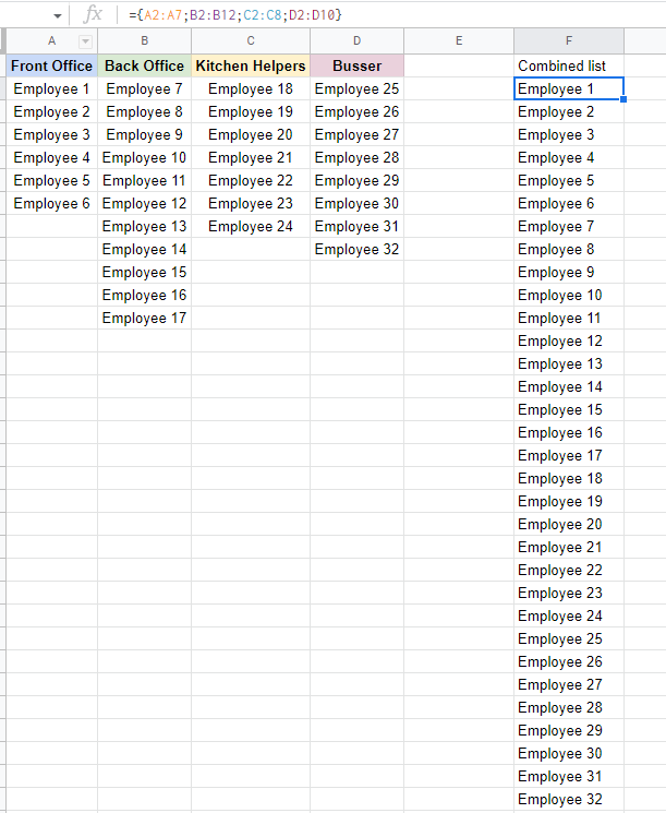
Consider the case of our restaurant again. Many restaurants break up schedules or shifts based on position. It can look like this:

If the manager wants to combine those names into one column for all their employees, they can use the Stacking Columns functionality.
In Google Sheets, you can combine stacks using the command “{range1;range2;range3; [etc…]}” The result will look like this:
You may use formulas, VBA programming, or macros to use this function in Excel. However, both methods would be cumbersome and hard to understand, so I don’t recommend them for non-data analysts. The macro is better used to copy/paste and then change the columns and fields.
Application: This command is excellent when merging multiple data sets into one column. Combining employee names, addresses, order numbers, or other like-criteria scattered across multiple columns becomes easier with this one formula.